Fixing the Early Data Bias in Bitcoin’s Power Law


The power law is one of the most widely used models in Bitcoin modelling.
But two hidden assumptions quietly distort the results:
1. We assume Bitcoin’s statistical clock started on Genesis Day (3 January 2009), and
2. We unintentionally overweight early data while effectively ignoring recent price action.
As you’ll see in this article, correcting these two issues dramatically improves the power law model — producing a cleaner fit and more realistic forecasts for Bitcoin’s future.
How the Bitcoin Power Law Became One of the Most Influential Models
I’ve been banging on about optimising the power law Day 0 since August 2024.
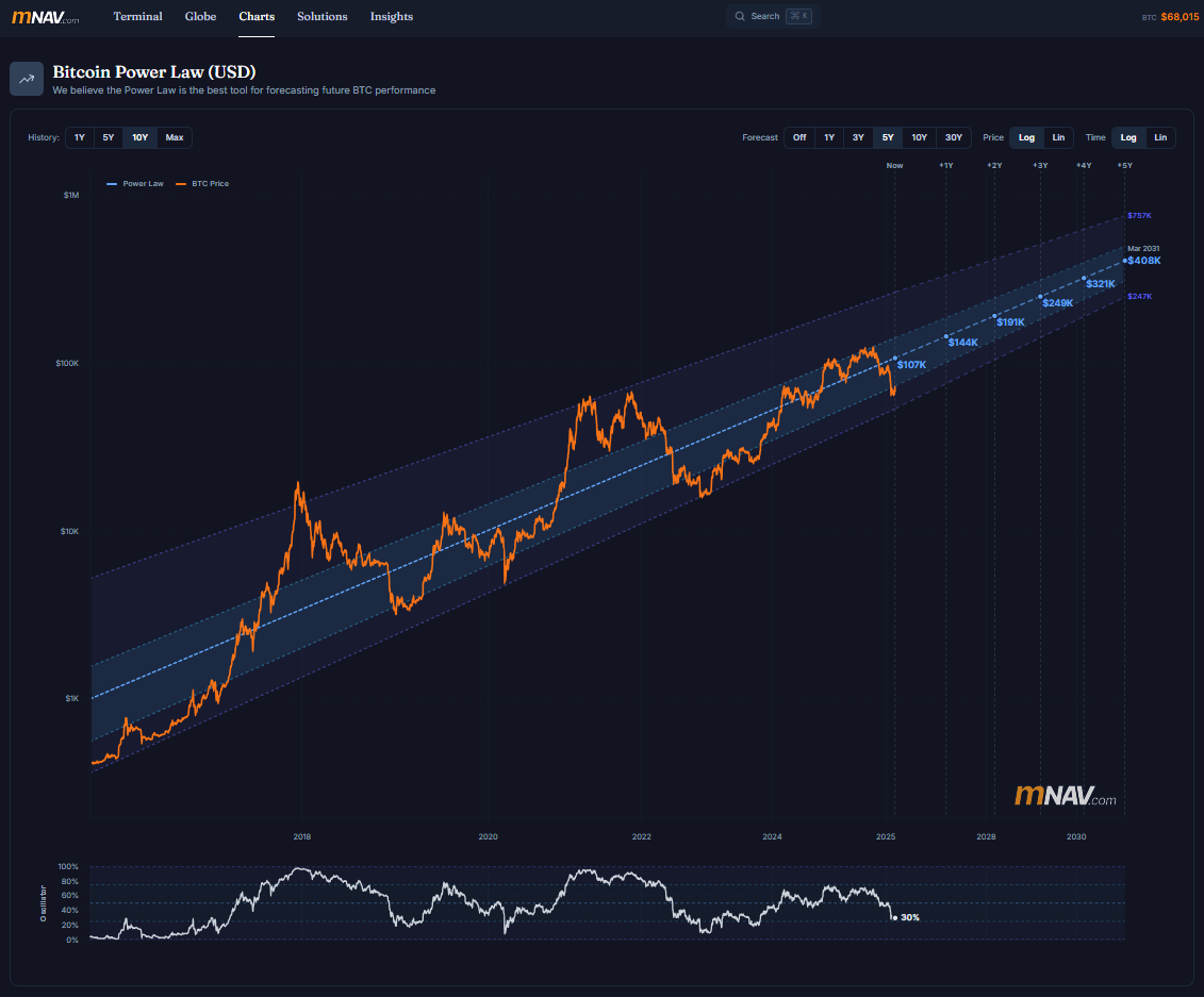
Our live mNAV.com power-law chart has incorporated this since it launched.
But recently, others have started to take notice.
About a month ago, Plan C started an X chat with BTCAnalytica and me to chat about how we could make sense of the fact that bitcoin has been much less volatile than recently, at least to the upside.
Since then, many charts and ideas have been shared as we’ve worked to understand why the power-law model forecasts have underwhelmed lately. I’ve rewritten this article from scratch three times.
Flowing from this discussion, BTCAnalytica published a paper pointing out the limitations of the power-law regression most people use and how it has continued to disappoint.
Plan C’s research also identified the bias introduced to the model when converting time to a log scale and how we can straighten it using Jacobian weightings.
I understand that Plan C will be releasing his updated quantile model shortly, but in this article, I wanted to lay out what I’ve learned to inform our improved power-law modelling, incorporating both updates, which sets the foundation for all our other models.
The Original Power Law: One of Bitcoin’s Most Elegant Patterns
The base-case Bitcoin power law, first identified by Giovanni way back in 2014, when Bitcoin was only five years old, is a thing of beauty!
Bitcoin’s price action is highly volatile, but when plotted on a log-log scale, we see a strong upward trend, with an astounding R2 of 0.96.
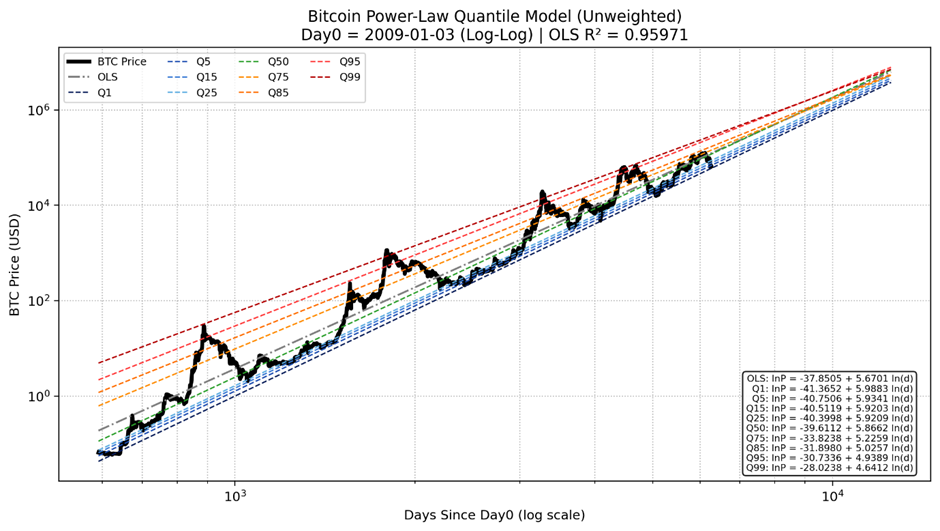
Bitcoin’s price grows roughly in proportion to the power of time, which appears as a straight line when plotted on log-log axes.
Many things in nature follow power-law growth trajectories.
Despite the name, Bitcoin’s power law is not a physical law of nature.
Like any model, it’s not perfect, but it’s useful.
It’s simply an empirical model describing how Bitcoin’s market value has evolved over time.
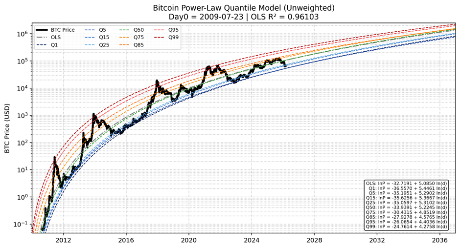
Quantile Regressions Define the Channel
In 2022, Plan C began incorporating the quantile regression into the power-law trend, which gave us a better sense of the range Bitcoin may continue to trade in.
The power-law trend alone tells us the centre of Bitcoin’s historical growth trajectory, around which Bitcoin oscillates.
Quantile regression allows us to estimate the range Bitcoin has historically traded within — from deep bear-market capitulation (Q1–Q5) through to cycle mania (Q95–Q99).
This transforms the model from a single line into a probabilistic channel that can help investors anchor expectations for likely ranges around the trend as Bitcoin grows.
The quantile modelling also highlights that Bitcoin's volatility oscillations have been compressing with time. But, to date, this has been hard to capture accurately with the current assumptions.
Is Genesis Day Really Bitcoin’s Statistical Birthday?
A key building block of the power law was the assumption that, like the Big Bang, everything started on 3 January 2009, Bitcoin’s Genesis Day, when the first bitcoin was mined.
The x-axis of the power law is the number of days since the assumed Day 0.
But the reality is, Bitcoin was really just a science experiment on Satoshi’s hard drive for the first few months.
· The second block wasn’t mined until a few days later.
· Bitcoin didn’t really act as a store of value or undergo true price discovery until it was traded on Mt Gox on 18 July 2010.
· In the middle of all this, in October 2009, Bitcointalk forum user NewLibertyStandard published the first formula-based BTC price based on the cost of electricity required to mine it.
So, rather than 3 January 2009 being bitcoin’s birthday, we view it more as the day it was conceived, with its real statistical birthday occurring later.
So when was Bitcoin’s real birthday?
The data gives us some clues.
The chart below shows R2 for possible Day 0s in 2009.
• The blue line shows that we maximise the OLS R2 when Day 0 is set to 22 July 2009.
• The orange line shows that the assumed day 0 has a significant impact on the model.
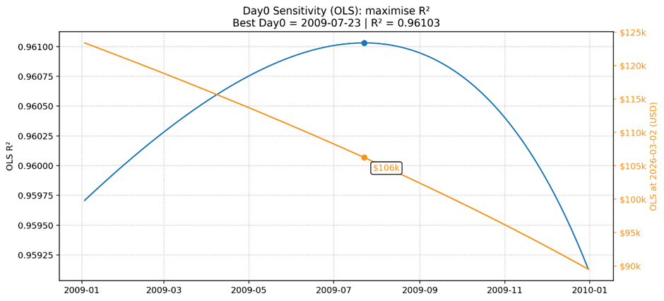
The choice of Day 0 has a significant impact on the predicted Bitcoin price.
• If we assume Day 0 = 3 Jan 09, then the OLS trend is $123k; if Day 0 shifts to the end of 2009, this drops to $90k.
• Meanwhile, the Goldilocks Day 0 (23 July 2009) gives us a current OLS trend of $106k.
We’ve been using this optimized OLS regression approach for a while now to identify the Day 0 for Bitcoin power-law modelling, but as you’ll see, fixing the distortion that the log-scale regression introduces.
The Hidden Problem with Log-Log Regression
Not only does shuffling the Day 0 forward give us a more realistic forecast, but it also makes the charts look even more satisfying, at least in the log-log scale. The early quantile regressions are neat, and they no longer cross (at least as early) future years.
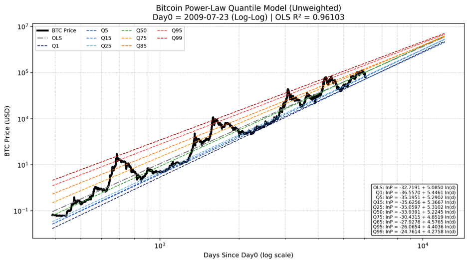
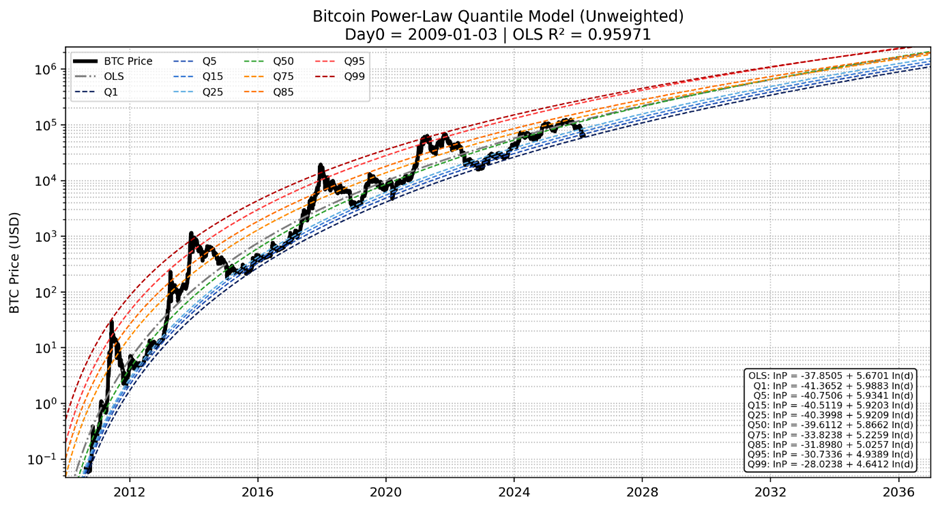
But the remaining problem is that the R2 is now optimised on the log-log scale, with a squashed time axis, which means we overweight the early data and therefore underweight the later data. This means everything looks great on the log-log scale, but the normal time price chart is still a bit messy.

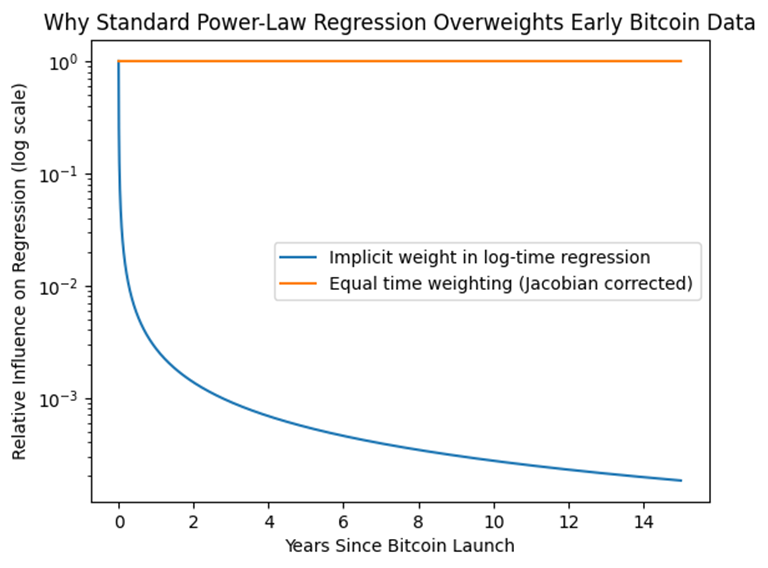
Most people don’t intuitively understand the log-time bias problem.
• In a log-time regression, the earliest data has a massively more influential effect.
• Later years contribute almost nothing to the regression.
• Jacobian weighting restores equal influence across time.
In simple terms:
• Without correction, 2009–2011 dominates the model.
• With correction, the prices across all of Bitcoin’s life are weighted equally.
In 2025, many people were holding out for a Bitcoin cycle top of $280k or so, which never came. These two corrections to the model help us understand why this occurred and enable us to better plan for the future.
With these tweaks, the improved Bitcoin model considers the more recent data, which has been less volatile. As more data arrives, the model will continue to adapt, weighing all information equally.
But What About Scale Invariance?
The original power-law framework draws inspiration from natural systems such as cities, river networks, and microbial growth that exhibit scale-invariant behaviour. The refinement proposed here does not challenge that idea. Instead, it addresses a statistical artifact introduced when performing regressions in log–log space.
Because each decade occupies the same width on a log axis, early data points receive disproportionately large influence on the regression slope. Applying a Jacobian weighting restores equal influence per unit of real time — a correction commonly used in physics, econometrics, and survival analysis when transforming coordinate systems or probability densities.
If Bitcoin truly follows a scale-invariant power law trajectory, the correction should not materially alter the long-term trend. But if early experimental data were dominating the regression, the adjustment provides a more balanced estimate of the underlying relationship.
Interestingly, once the weighting bias is removed, the optimal Day-0 consistently falls in late 2009 — the period when Bitcoin first acquired a measurable market price tied to the cost of mining it.
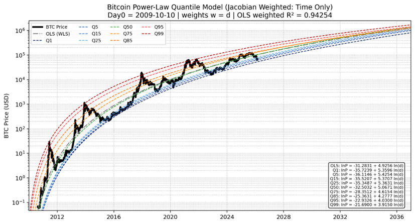
The Jacobian Fix: Giving Each Year of Bitcoin Equal Weight
To explain this another way, on a log-time axis, Bitcoin’s first year occupies a huge portion of the chart, while the most recent years are compressed. That means the regression “cares” much more about the early data than the recent data, even though the market today is far more mature with a much larger market cap.
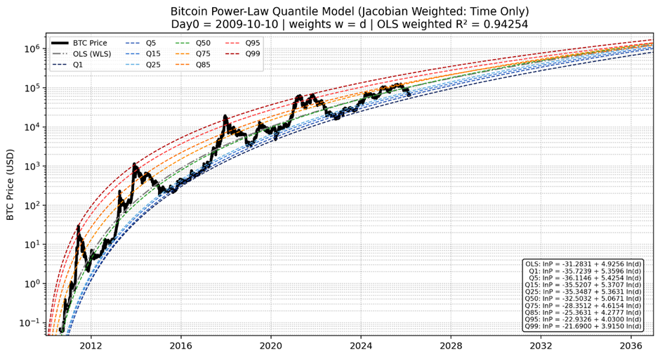
As shown in the chart below, this makes the quantiles look messier on the log-log chart.
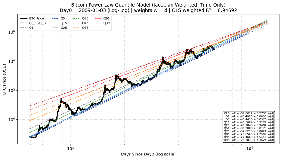
However, on the normal time scale, with the Jacobian weighting added to the regression, the quantiles are neater across the full spectrum and into the future.
Jacobian weighting ensures that each year of Bitcoin’s history contributes equally to the regression, rather than letting the earliest years dominate the model.
Jacobian weighting doesn’t manipulate the regression outcome; it simply reverses the distortion introduced by log-transforming time.
Without this correction, the early years of Bitcoin implicitly receive far more weight in the regression than the later years. Applying the Jacobian weightings restores equal influence to each unit of time in the original scale.
While these charts use Genesis Day, in the next section, we’ll look at how we can also optimise Day 0 using the normal time space.
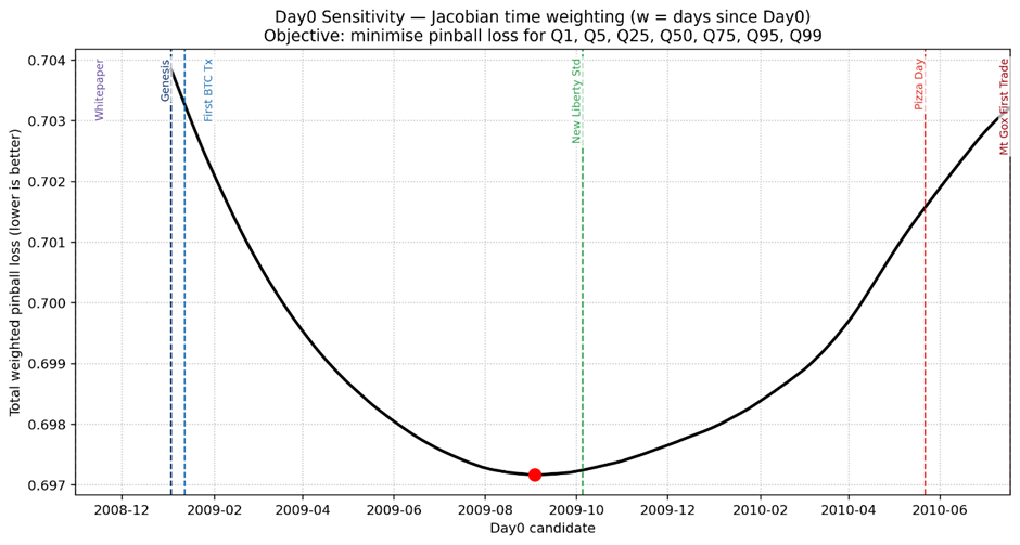
Let the Data Decide: Optimising Day-0 with Quantile Pinball Loss
Quantiles are determined using a statistical concept called ‘pinball loss’. Rather than simply using the OLS regression, we can also use the pinball loss approach to optimise the quantile regression channel.
The caveat here is that the Day 0 we end up with is highly influenced by the quantiles considered. Our strong preference is to provide a conservative forecast, tailored to the more recent years with lower volatility, and avoid disappointment due to excess hopium.
In the first line of the table below, we see that if we just use the Q50 and minimise pinball loss (i.e. what is the day 0 that gives us 50% of the data above and 50% below the trend line) we get an optimal day 0 of 21 July 2009, which is very similar to what we got previously when we optimised to maximise R2 with the OLS trend line.
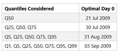
But rather than just the trend, we also care about the quantiles, or the long-term channel that Bitcoin follows. As we add more quantiles to the Day 0 optimisation, we get a later Day 0, and thus a less bullish overall projection.
If we consider four quantiles above and four equally spaced quantiles below the trend, we get an optimal Day 0 of 3 September 2009. As shown in the chart below, the optimal Day 0 lies between Genesis Day and the time Bitcoin was first traded on Mt Gox, and is pretty close to the time when NewLibertyStandard noticed that Bitcoin's price could be tied to the energy cost of mining.
The chart below shows the result when we optimise both the quantiles and Day 0 together. If you look closely to the left of this chart, you’ll see that the lower quantiles are bunched, and it doesn’t look as clean on the log-log scale.
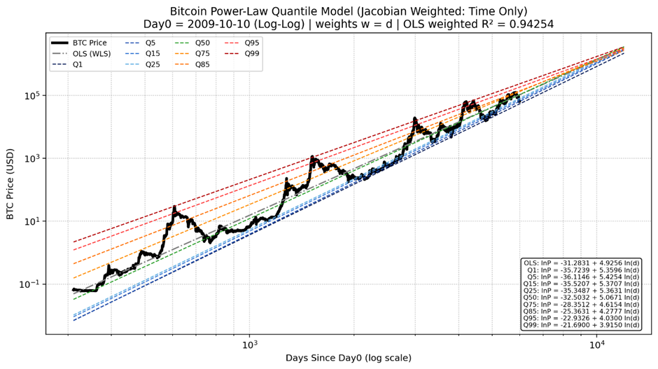
But we get a much cleaner chart when we pivot to a normal time scale. In recent years, the lower quantiles have been neat and parallel, while the upper quantiles have been falling towards the trend line in this model without collapsing.
Overall, while no model is perfect, we think this version is a significant improvement, particularly for modelling recent and future Bitcoin price action.
How These Adjustments Change Bitcoin’s Forecast Range
So what does this mean in practice?
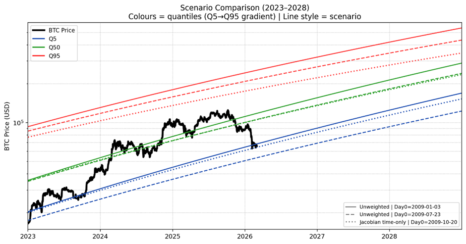
The chart below shows that:
· Pushing day 0 drops the Q50 for both the unweighted and weighted scenarios, meaning people who use our mNAV power law chart are less likely to get wrecked on hopium.
· At the lower end, the time-weighted and day 0 optimised version is fairly similar to the original model. Because it better models recent tighter volatility, the forecast low is higher.
· Meanwhile, at the upper end, pushing the day 0 brings down the upper quantile forecasts, and correcting the time scale brings this down even further.
· Overall, we get a less bullish trend due to the later Day 0 and a tighter channel, with less upside volatility, while the floor remains similar.
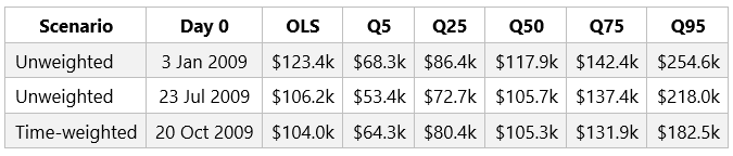
The table below shows the numerical implications of the different models, again showing how pushing Day 0 back brings down the trend while correcting for the time distortion compresses the forecast range to something more sensible.
Is this just curve fitting?
A fair criticism whenever we refine a robust base model is that we may simply be “fitting the past.”
But the adjustments made here are not arbitrary tweaks to maximise price predictions. Instead, they correct two structural issues in the standard model:
1. the arbitrary choice of Genesis Day as Day-0, and
2. the mathematical distortion introduced when time is log-transformed.
In other words, the goal isn’t to make Bitcoin look more bullish — it’s to remove biases in the modelling framework so the regression more accurately reflects how the data actually evolves over time.
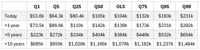
Where Bitcoin Sits in the Power-Law Range Today
Ultimately, everyone wants to know where we are now relative to the range and where we could be headed. Unfortunately, no model can tell you where BTC is going, but some realistic ranges can help to keep our expectations, along with fear and greed, in check.
Why This Matters
These refinements matter because many investors use the power law as a mental anchor for Bitcoin’s long-term trajectory.
If the model systematically overestimates future upside, it can lead to unrealistic expectations and poor decision-making.
A more balanced model helps investors frame realistic scenarios across both bull and bear regimes.
A Cleaner Power Law for the Next Phase of Bitcoin
Bitcoin’s power law remains one of the most elegant empirical models in the space.
But like any model, small tweaks to fundamental assumptions can have large consequences.
By optimising Day-0 and correcting the log-time distortion, we end up with a framework that better reflects Bitcoin’s full history — particularly the more recent regime where volatility has gradually compressed.
The result is a power-law model that is less prone to unrealistic upside expectations while still capturing Bitcoin’s long-term exponential growth.
Of course, no model can perfectly predict the future. But refining the assumptions behind the power law can help anchor expectations and keep both fear and greed in check.
Bitcoin’s power law remains one of the most elegant empirical models in the space. But as Bitcoin matures, the assumptions behind the model need to mature as well.