From Time to Work: Rethinking Bitcoin’s Power Law

There’s no such thing as a perfect model, but some are better than others.
In the case of Bitcoin, the power law appears to be the most effective approach for understanding its future trajectory.
Most people simplistically model Bitcoin’s price trajectory since Genesis Day (3 January 2009). However, we can make subtle adjustments to improve the model's accuracy and robustness.
In our previous article, we showed how we can optimise Bitcoin’s Day 0 using only price data to improve the power-law model.
In this article, we examine the data more closely and find that Bitcoin’s market cap is most closely linked to its block height, or the work that has gone into it.
When we account for Bitcoin’s changing issuance rate (due to halvings) and the volatile first few years of mining, we obtain a significantly better model fit.
We can then convert this back to time vs price and obtain a more accurate prediction than price alone. This may sound like we’re splitting hairs, but it makes a material difference to the forecasts.
The Hidden Flaw in Time-Based Bitcoin Models
The first challenge overlooked by simplistic time-based Bitcoin models is the instability of the mining network in Bitcoin’s early years.
Although the Genesis Block (Bitcoin’s block 0) was mined on 3 January 2009, block one was not mined until 9 January 2009. And, as shown in the chart below, the target rate of one block every ten minutes did not stabilise until around year two.
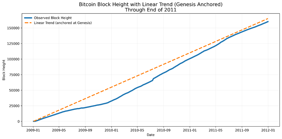
In the earliest months, Bitcoin was mined mainly by Satoshi, using a single CPU (before ASIC miners). It appears that the early hat hardware was insufficient to achieve the protocol’s intended block cadence of one block every 10 minutes (144 blocks per day).
Thus, when we assume that “time since genesis” is a clean independent variable, we inadvertently introduce distortions that echo through the power law (log-log) regressions that can be avoided if we tie the power law regression back to block height (i.e., proof of work).
Proof-of-Work as Bitcoin’s Native Timekeeper
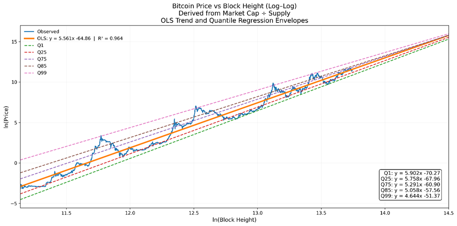
Rather than simplistically modelling time versus price, plotting block height versus market cap yields a substantially improved fit, with an R² of 0.970 (versus R² = 0.960 for a standard price-based power law anchored at the Genesis Date). While both models are robust, with high R2 values, the quantile projections for the block height-based regression are clean, with no overlap across future years.

Network Value Tracks Work, Not the Calendar
Most people are interested in Bitcoin’s price, not market cap, which introduces another error that degrades model accuracy because Bitcoin’s supply is not constant.
As the chart below of cumulative BTC supply shows, the issuance rate changes discretely at each halving. This uneven growth in supply distorts price-only models.
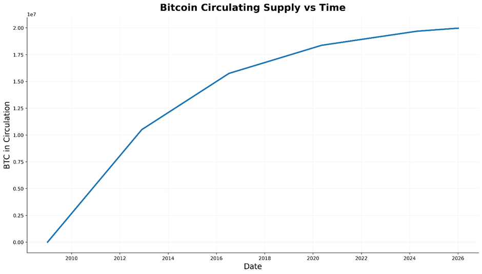
The effect of the halvings will ultimately diminish as their impact wanes, but the non-linear issuance has a significant effect if we assume that Bitcoin’s price follows a simple power law in the early days.
Fortunately, it’s easy to determine price from market cap:
price = market cap / current circulating BTC supply
Converting market capitalisation to price using the known supply schedule preserves the structural advantages of the block-height model along with the changing issuance schedule while allowing us to work in familiar price terms. Even after converting to price, the quantile regressions are tidy, with no overlap in future years.
Converting Back to Standard Time
We can then map block height back to calendar time using the observed block-height-time relationship.
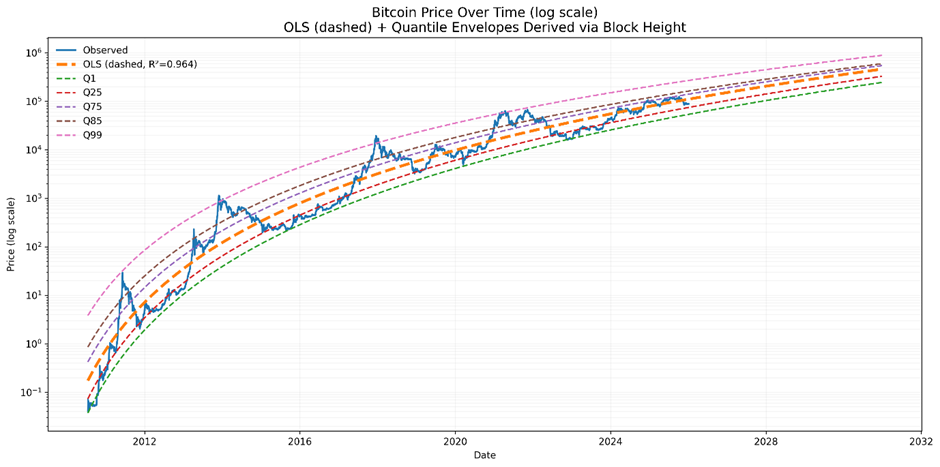
A particularly key feature of the block height/market cap model is the uniformity of the quantile bands. In price-only power laws (as shown below), quantiles are typically lumpy and bulging in the early years and overlap in the later years.
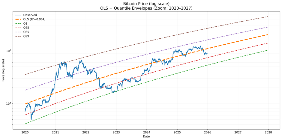
When we zoom in to the present, the block-height model is still clean and implies a current trend price of $102k.
Model Comparison
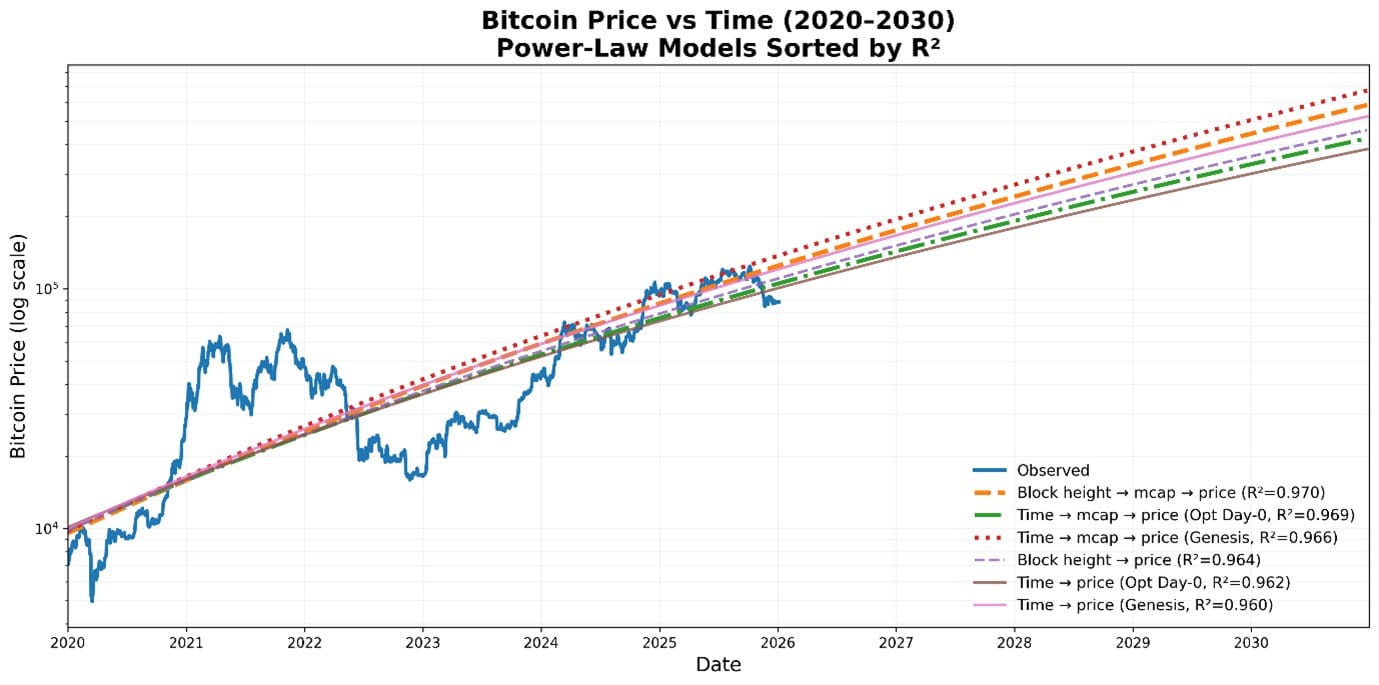
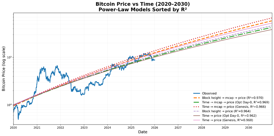
While it might seem like we’re splitting hairs, when we zoom in, we can see that the different models produce different results.
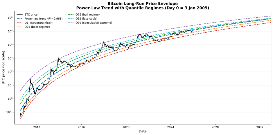
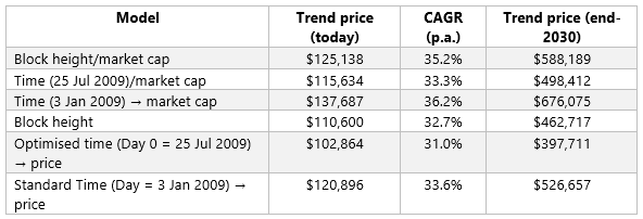
The chart below shows the block height/market cap-based model (converted to price) (R2 = 0.970) along with five other models. The good news is that the most accurate model is the second most bullish.

The table below shows the implications on the trend price, CAGR, and forecast trend price at the end of 2030.
Which Model is Best?
The answer really is ‘it depends’.
The price-based power law using the Genesis Day is the simplest to calculate and understand; however, for accurate forecasting, the block-height vs. market-cap version is more robust. The optimised day 0 version is between the other two and more conservative/less bullish.
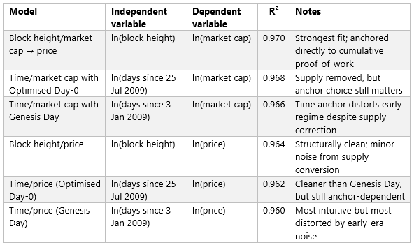
The table below summarises the models by R2, ordered from highest to lowest.
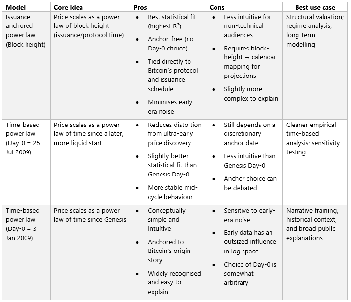
The table below lists the pros, cons, and use cases of the different models.
Ultimately, there is no perfect model, and numerous variations of the power law.
· Starting from block high vs market cap data appears to be the most robust approach,
· Price vs time with starting from Genesis Day, is the simplest, while
· Optimising Day 0 lies somewhere in between.
The Case for Block Height as Bitcoin’s Valuation Spine
In summary, time-based power laws are intuitive and useful, but they suffer from an unavoidable flaw: they require an arbitrary anchor.
Block height avoids this problem entirely. By anchoring valuation to Bitcoin’s native clock — cumulative proof-of-work — the block-height model:
· removes subjective assumptions,
· aligns directly with protocol economics,
· delivers the strongest statistical fit,
· and produces stable, well-behaved long-term projections.
Time-based models remain valuable as bounds and narrative tools. However, for long-term structural valuation, block height provides the cleanest and most robust power-law framework.